This is the first in a series about using Python and Jupyter notebooks to explore astronomy, diving into the interesting calculations, methods, and visualizations used in this field.
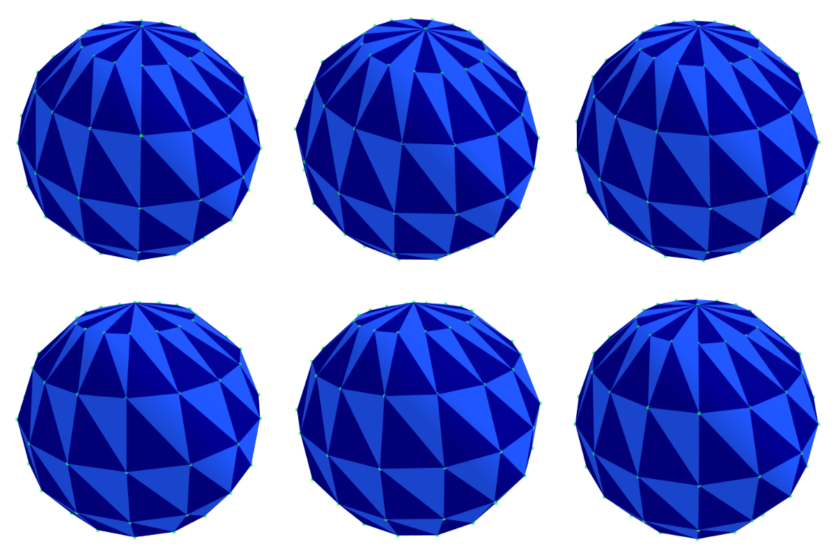
We will begin by defining and visualizing planet-like shapes (spheroids). The code to accompany this tutorial is on github. Below is an example visualization:
Loading Utilities
I use plotly and moviepy to create some helpful utilities to plot the 3D meshes defined here, and to stich together renderings of these meshes into .gif files that can be easily embedded into web content.
Create the following directory structure in your project to setup these utilities, with an empty __init__.py file to tell python we are creating a module.
project
└───plot
|   │   __init__.py
|   │   plotly_utils.py
<other project files>
Create plotly_utils.py and populate it with the following contents:
import io
from PIL import Image
import numpy as np
import plotly.graph_objects as go
import moviepy.editor as mpy
from scipy.spatial.transform import Rotation as R

def show_poly_3d(nodes=None, polys=None, show_nodes=False):
    '''
    Makes a basic invokation of __plot to show a single frame
    '''
    fig = __plot(nodes=nodes, polys=polys, t=0, show_nodes=show_nodes)
    fig.show()
    return

def create_poly_3d_gif(filepath, nodes=None, polys=None, fps=15, duration=8, show_nodes=False):
    '''
    Creates a gif using moviepy from frames built using plotly
    '''

    def make_frame(t):
        return __plotly_fig2array(__plot(nodes=nodes, polys=polys, t=t, fps=fps, duration=duration, show_nodes=show_nodes))

    gif_output_file = filepath
    animation = mpy.VideoClip(make_frame, duration=duration)
    animation.write_gif(gif_output_file, fps=15, loop=0, opt="OptimizePlus", fuzz=10)
    animation.close()

    # forcing garbage collection here seems to account for a 'bug' in moviepy loop count encoding
    import gc
    del animation
    gc.collect()

    return

def __plotly_fig2array(fig):
    '''
    Convert plotly figure into an 2x2 array of RGB bytes
    '''
    fig_bytes = fig.to_image(format="png", scale=1.0, engine='orca')
    buf = io.BytesIO(fig_bytes)
    img = Image.open(buf)
    return np.asarray(img)


def __plot(nodes=None, polys=None, t=0, fps=15, duration=8, show_nodes=False):
    '''
    Creates a plotly figure for a single frame, displaying nodes with scatter3d and
    nodes + polygons with mesh3d
    '''
    assert nodes is not None, "nodes is a required parameter"
    if polys is None:
        show_nodes = True  # always show nodes if there are no polys

    # rotate the polygon on each frame
    frame = t*fps
    max_frame = fps * duration
    p = ((frame - 1) / (max_frame))
    roll = -(2*np.pi/8) * p
    pitch = -np.sin( 2*np.pi * p + 0.321) * (np.pi / 32)
    rotated = R.from_rotvec([pitch, 0.0, roll]).apply(nodes)

    # populate the plot's contents
    data = []
    if polys is not None:
        data.append(__get_mesh3d(rotated, polys))
    if show_nodes:
        data.append(__get_node_scatter3d(rotated))

    # initialize the plot
    fig = go.Figure(data=data)
    fig['layout']['margin'] = dict(l=0, r=0, b=0, t=0)
    fig["layout"]["height"] = 400
    fig["layout"]["width"] = 400

    # configure the plot's axes
    hide_axis_params = {
        'title': '',
        'autorange': False,
        'showgrid': False,
        'zeroline': False,
        'showline': False,
        'ticks': '',
        'showticklabels': False,
        'backgroundcolor': "rgba(0, 0, 0, 0)",
        'showbackground': True,
    }
    fig["layout"]["scene"] = {
      'aspectmode': 'cube',
      'xaxis': {
          **hide_axis_params,
          'range': [np.min(nodes[:,0]), np.max(nodes[:,0])*1.1]
        },
      'yaxis':{
          **hide_axis_params,
          'range': [np.min(nodes[:,1]), np.max(nodes[:,1])*1.1]
       },
      'zaxis': {
          **hide_axis_params,
          'range': [np.min(nodes[:,2]), np.max(nodes[:,2])*1.1]
        }
    }

    # configure the camera to be more zoomed in
    fig["layout"]["scene_camera"] = {
      'up': dict(x=0, y=0, z=0.8),
      'center': dict(x=0, y=0, z=0.0),
      'eye': dict(x=0.8, y=0.8, z=0.8)
    }

    return fig


def __get_mesh3d(nodes, polys, color=None):
    '''
    Constructs a plotly mesh3d object from a list of nodes and polygons
    '''
    i, j, k = zip(*polys)

    # determine colormap settings
    if color is None:
        colormap_settings = {
            'colorscale': [[0, '#010095'], [1, '#1F56FF']],
            'intensity': [c%2 for c in range(len(i))]
        }
    else:
        colormap_settings = {
            'colorscale': [[0, color]],
            'intensity': 0
        }

    return go.Mesh3d(
        **colormap_settings,
        x=nodes[:,0],
        y=nodes[:,1],
        z=nodes[:,2],
        intensitymode='cell',
        flatshading=True,
        i=i,
        j=j,
        k=k,
        showscale=False
    )


def __get_node_scatter3d(nodes):
    '''
    Constructs a plotly scatter3d object from a list of nodes
    '''
    return go.Scatter3d(
        x=nodes[:,0],
        y=nodes[:,1],
        z=nodes[:,2],
        mode ='markers',
        marker = dict(
            size = 3,
            color = '#CC0000',
            opacity = 0.7
        )
    )
Notebook Setup
Create a file called requirements.txt with the following contents:
moviepy==1.0.3
numpy==1.22.4
Pillow==9.1.1
plotly==5.8.2
scipy==1.8.1
nbformat==5.4.0
decorator==4.4.2
kaleido==0.2.1
Install the dependencies. This examples assumes the usage of miniconda, but you can use your own environment manager to install the dependencies listed above.
Run the following commands:
conda create -n "astro" python=3.9 --file requirements.txt
conda activate astro
Create and start a notebook globe_mesh_uv.ipynb, and activate the astro conda environment.
Inside globe_mesh_uv.ipynb, import the notebook prerequisites. Make sure that you properly added the plotting module mentioned above into the plot/ folder.
import numpy as np
from itertools import product
from plot.plotly_utils import show_poly_3d, create_poly_3d_gif
Define an approximation to the earth’s shape (oblate spheroid)
We will use parameters from the World Geodetic System (WGS 84):
We exaggerate the oblateness of the earth to make the shape more obvious in our visualizations.
OBLATENESS_EXAGGERATION = 1.25

# WGS-84 parameters
A = 6378137 * OBLATENESS_EXAGGERATION  # meters
B = 6356752.3142  # meters

def spheroid(lat, lon):
    '''
    Spheroid surface defined in spherical coordinates (latitude / longitude).
    Returns points on the spheroid in 3D X/Y/Z coordinates
    '''
    return np.array([
        A*np.cos(lat)*np.cos(lon),
        A*np.cos(lat)*np.sin(lon),
        B*np.sin(lat)
    ])
Define the Mesh Nodes
We will combine concepts of a UV Sphere and the Geographic Coordinate System to construct our spheriod mesh.
The mesh nodes are created by sampling spheroid() over a grid of latitude / longitude values.
def uv_sphere_nodes(n_lat=8, n_lon=15):
    nodes = []

    # create the nodes
    latitudes = np.linspace(np.pi/2.0, -np.pi/2.0, num=n_lat, endpoint=True)
    longitudes = np.linspace(-np.pi, np.pi, num=n_lon, endpoint=False)

    # top point
    nodes.append(spheroid(latitudes[0], 0.0))

    # middle points
    for lat, lon in product(latitudes[1:-1], longitudes):
        nodes.append(spheroid(lat, lon))

    # bottom point
    nodes.append(spheroid(latitudes[-1], 0.0))

    return np.array(nodes)
Visualize the Nodes in 3D
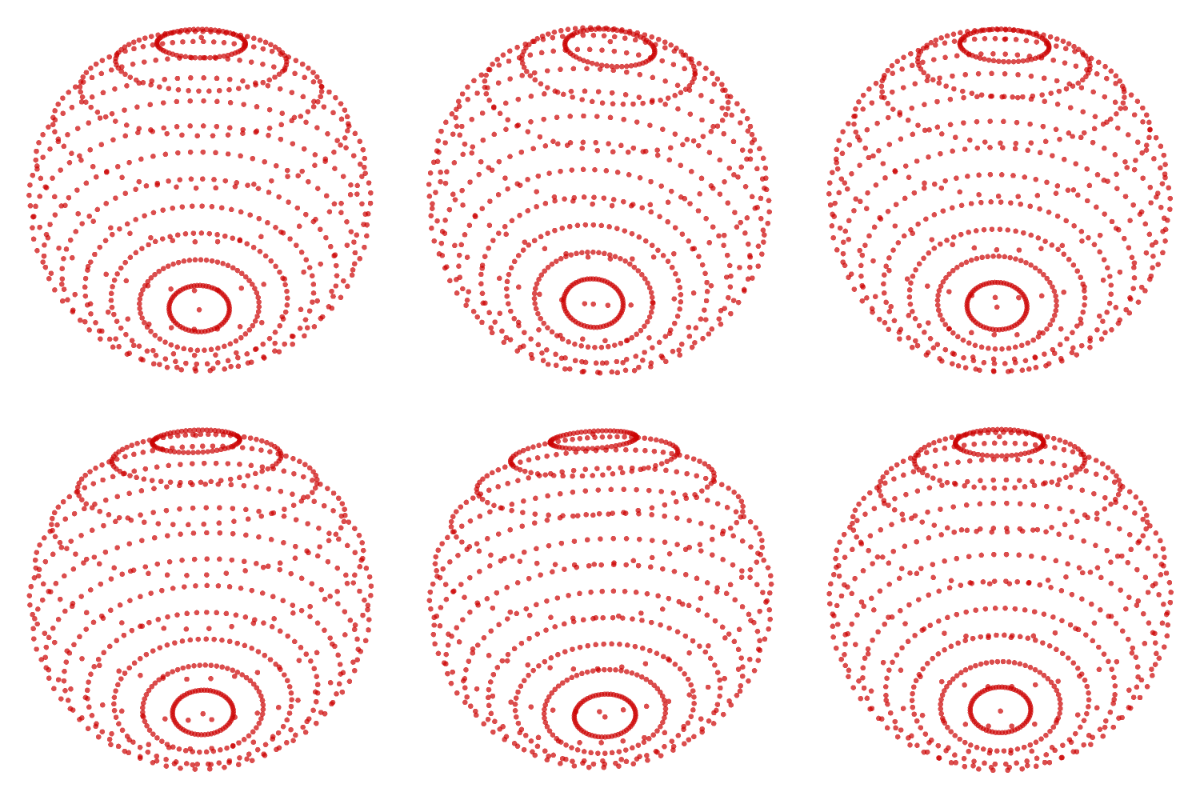
The plotting utilities can be used to visualize the nodes.
To show the nodes:
show_poly_3d(nodes=uv_sphere_nodes(n_lat=15, n_lon=60))
To generate a .gif of the nodes with a rotating animation to illustrate the 3d perspective:
create_poly_3d_gif('./image/uv_spheroid_nodes_dense.gif', nodes=uv_sphere_nodes(n_lat=15, n_lon=60), duration=2)
The resulting .gif:
Adding Polygons
Create a low-density set of nodes for illustrative purposes:
N_LAT = 8
N_LON = 15
nodes = uv_sphere_nodes(n_lat=N_LAT, n_lon=N_LON)
The mesh’s polygons are defined by defining connections between groups of three nodes. We will define the UV spheroid from three types of polygon: top, middle, and bottom.
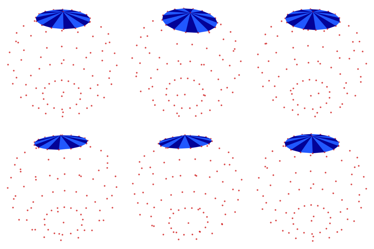
Top-Row Polygons
Define the top polygons by connecting each edge in the first line of latitude with the top node:
top = [[0, j + 1, j + 2] for j in range(N_LON-1)]
top.append([0, N_LON, 1])

show_poly_3d(nodes=nodes, polys=top, show_nodes=True)
Middle-Row Polygons
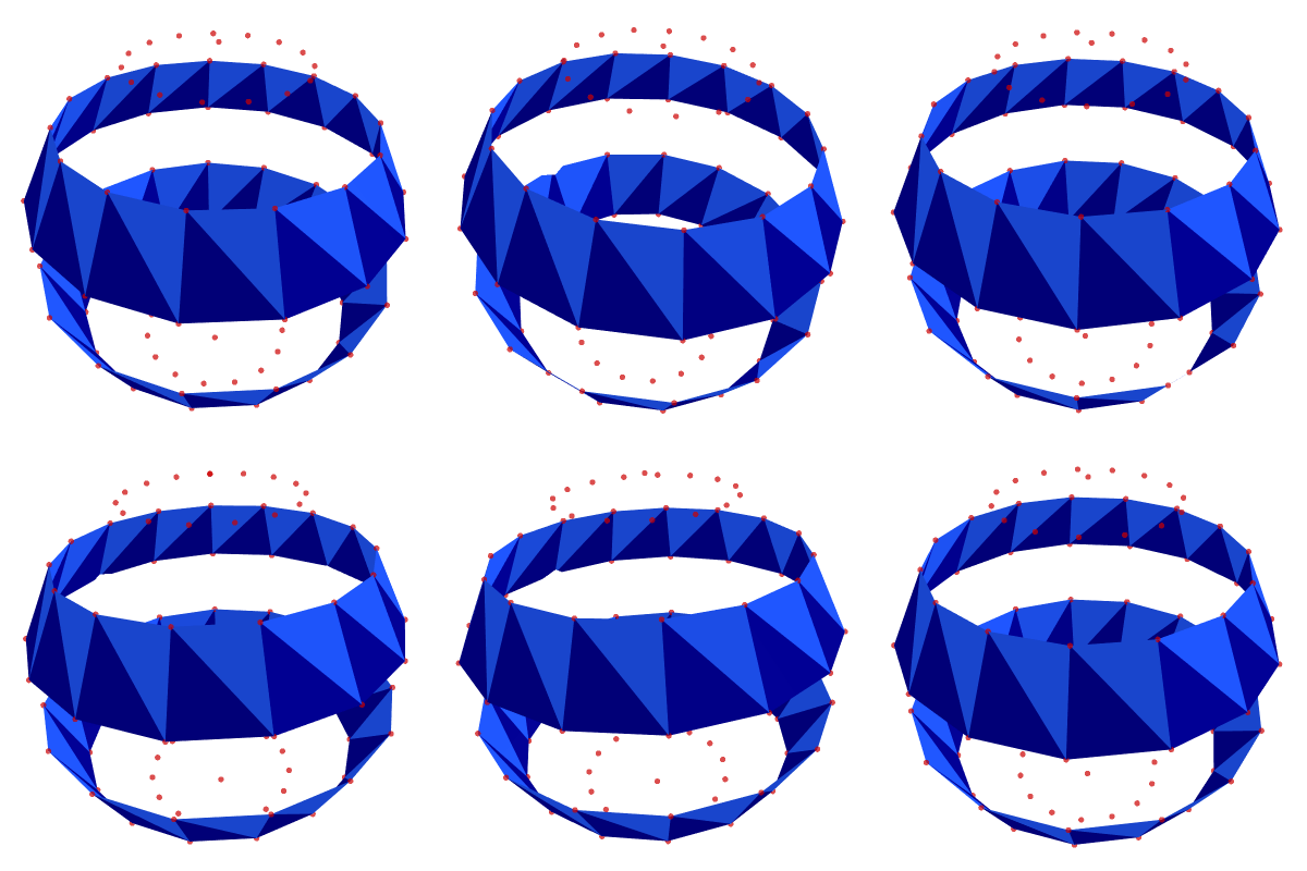
Define the middle polygons by subdividing each quadrilateral face between not-terminal parallels:
middle = []
for i in range(1, N_LAT-2):
    for j in range(N_LON - 1):
        middle.append([(i-1)*N_LON + j + 1, i*N_LON + j + 1, i*N_LON + j + 2])
        middle.append([(i-1)*N_LON + j + 1, i*N_LON + j + 2, (i-1)*N_LON + j + 2])
    middle.append([i*N_LON, (i+1)*N_LON, i*N_LON + 1])
    middle.append([i*N_LON, i*N_LON + 1, (i-1)*N_LON + 1])

# plot only every other band
alternating_bands = [band for i, band in enumerate(middle) if (i//(2*N_LON))%2]

show_poly_3d(nodes=nodes, polys=alternating_bands, show_nodes=True)
Bottom-Row Polygons
Define the bottom polygons similarly to the top:
bottom = [[(N_LAT-3)*N_LON + j + 1, (N_LAT-2)*N_LON + 1, (N_LAT-3)*N_LON + j + 2] for j in range(N_LON - 1)]
bottom.append([(N_LAT-2)*N_LON, (N_LAT-2)*N_LON + 1, (N_LAT-3)*N_LON + 1])

show_poly_3d(nodes=nodes, polys=bottom, show_nodes=True)
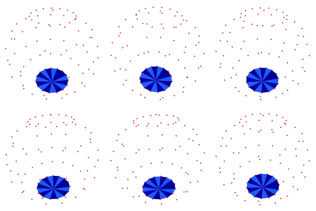
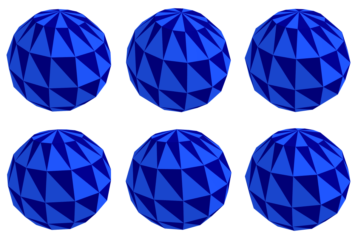
Putting the UV Sphere Together
polys = top + middle + bottom

show_poly_3d(nodes=nodes, polys=polys)
That’s it! The code to reproduce everything seen in this tutorial can be found on github. Please submit an issue if you have any problems running this code!

